
Implementation of diffusion models look hard? Do not fret - fortunately there’s no need to introduce fancy ML techniques to understand the underlying mechanisms. In this post I discuss how to learn a 2D synthetic dataset with a simple vanilla feed-forward network (or the nano diffusion). Code is provided.
Recap
In part 1 of the series on diffusion models, I described how the Smoluchowski equation is really the foundation for diffusion models. These days, they became indispensable in the state-of-the-art image generation with many good resources available on the topic. These achievements are possible by the use of a number of advanced ML techniques which are very useful but can overwhelm the unitiated and obfuscate the fundamental mechanisms. In this part, I strip down diffusion to its bare minimum and highlight the essentials.
Nano diffusion
Instead of multi-dimensional image datasets, I present a simpler problem of learning the diffusion model on a 2D synthetic dataset. The neural network is a shallow feed-forward neural network. For those interested in the pytorch code, check out the notebook.
Specyfing the dataset
First let’s specify the dataset:
def gen_x0(n = 2,scale = 200,n_samples=128):
    x0 = 2*torch.rand(n_samples,n)-1
    x0 /= torch.sqrt(((x0)**2).sum(axis=1,keepdim=True))
    x0 *= torch.distributions.gamma.Gamma(concentration=scale,rate=scale).sample((n_samples,1))
    return x0
It is concentrated on a ring of radius 1 with nonuniform angular density. The ring thickness is controlled by the scale parameter. We show a 2D histogram of the dataset, 1D radial and 1D angular histograms:
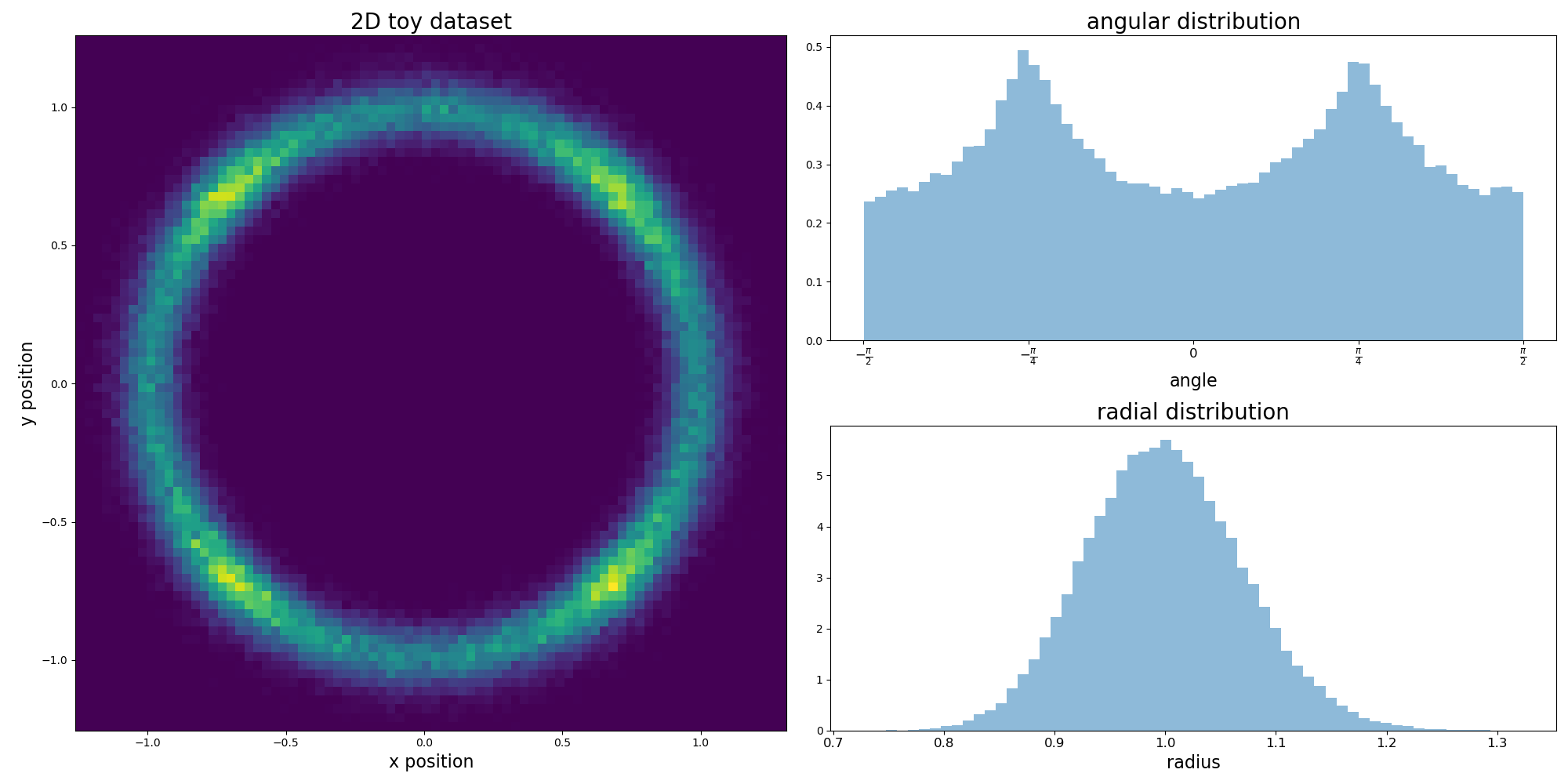 Toy dataset
Forward process
The Langevin equation for the forward process is the continuous version considered in the seminal paper:
\[\frac{d}{dt} x(t) = - \frac{1}{2} \beta(t) x(t) + \sqrt{\beta(t)} W(t), \qquad t \in (0,T)\]
where the noise schedule is linear \(\beta(t) = \beta_- + (\beta_+ - \beta_-) \frac{t}{T}\). At first it looks quite arbitrary but this process has few advantages:
- the noise is added in a relatively small amounts, especially near \(t = 0\),
- a linear drift \(-\frac{1}{2} \beta(t) x(t)\) admits both an analytic solution to the transition kernel used in the learning process:
\[p(x,t; x_0,0) \sim \exp \left ( - \frac{(x - A(t) x_0)^2}{2B(t)^2} \right ),\]
as well as an explicit sampling formula:
\[x(t) = A(t) x(0) + B(t) \epsilon,\]
with \(A(t) = \exp (-\frac{1}{2} \int_0^t \beta(t') dt')\), \(B(t) = \sqrt{1 - A(t)^2}\) and \(\epsilon \sim N(0,1)\) drawn from a normal distribution.
The function for generating a forward process reads:
def forward_x(x0,t):
    A = np.exp(-1/2*(beta_min*t + 1/(2*T)*(beta_max-beta_min)*t**2))
    B = np.sqrt(1-A**2)
    noise = torch.randn_like(x0)
    return A*x0 + B*noise, noise
Reverse process
The reverse process (matched with the forward process) is in turn the Langevin equation:
\[\frac{d}{dt} x(t) = - \frac{1}{2} \beta(t) x(t) - \beta(t) \partial_{x(t)} \log p_t(x(t)) + \sqrt{\beta(t)} W(t), \qquad t \in (0,T)\]
In this case, we start out from \(x(T) \sim N(0,1)\) drawn from a normal distribution and evolve to \(x(0)\). The key role of an additional drift term was discussed in part 1, we will see that it will become the part approximated by the neural network \(\partial_{x(t)} \log p_t(x(t)) \approx s_\theta (x(t),t)\). The function for the backward process reads (notice the sign change of the drift term due to non-standard time direction!):
def sample_sde(score_net, batch_size = 128, dt = 5e-3):

    def beta(t):
        return beta_min + (beta_max-beta_min)*t/T

    def reverse_step(xt,t):
        tmat = (torch.ones_like(xt)*t)[...,:-1]
        xt_new = xt + (1/2*beta(t)*xt+ beta(t)*score_net(xt,tmat))*dt
        xt_new += np.sqrt(beta(t))*torch.randn_like(xt)*np.sqrt(dt)
        return xt_new

    xt = torch.randn(batch_size,2)
    N = int(T/dt)
    for n in range(N,0,-1):
        xt = reverse_step(xt,n*dt)

    return xt
Neural network
The score_net passed to the reverse_xT function is the discussed neural network. To ease the discussion, we aim at the simplest network that does the job. So there will be no UNets here but a vanilla feed-forward network. The position x and time t parameters are simply concatenated before passing through the network:
class basic_net(nn.Module):
    def __init__(self, dim = 2, layer_size = 64, n_layers = 6):

        super().__init__()
        self.activ = nn.ReLU()

        self.layers = []
        self.layers.append(nn.Linear(dim+1,layer_size))
        for _ in range(n_layers-2):
            self.layers.append(nn.Linear(layer_size,layer_size))
        self.layers.append(nn.Linear(layer_size,dim))
        self.layers = nn.ModuleList(self.layers)

    def forward(self,x,t):

        xt = torch.cat((x,t),axis=-1)
        for i, l in enumerate(self.layers[:-1]):
            xt = self.activ(l(xt))
        xt = self.layers[-1](xt)

        return xt
Learning phase
In part 1 we discussed the loss function of the learning phase:
\[L(\theta) = E_{t\sim U(0,T)} E_{x(0)} E_{x(t)| x(0)} \left ( \lambda(t) \left \| s_\theta(x(t),t) - \partial_{x(t)} \log p(x(t), t; x(0),0) \right \|^2 \right )\]
The Langevin equation for the forward process has a known transition kernel \(p(x, t; x=x_0,t=0)\) so that the score function can be calculated explicitly:
\[\partial_x \log p(x, t; x=x_0,t=0) = - \frac{x-A(t) x_0 }{B(t)^2}\]
and moreover, we plug in the noisy sample \(x(t) = A(t) x(0) + B(t) \epsilon\) as a function of the noise \(\epsilon\). The loss function simplifies considerably:
\[L(\theta) = E_{t\sim U(0,T)} E_{x(0)} E_{\epsilon} \left ( \lambda(t) \left \| s_\theta\left (A(t)x(0) + B(t) \epsilon,t \right ) + \frac{\epsilon}{B(t)}\right \|^2 \right )\]
which now is sampled over the initial points \(x(0)\), the noise \(\epsilon\) and time \(t\). The interpretation is quite surprising – the resulting neural network \(s_\theta\) is trained to match a set of rescaled noise samples \(\epsilon\). The \(1/B(t)\) scale causes a training innstablility since \(1/B(t) \to \infty\) near \(t \approx 0\). To help with these convergence issues, we pick a weight function \(\lambda(t) = B(t)^2\). Full training loop is given below:
def A(t):
    return np.exp(-1/2*(beta_min*t + 1/(2*T)*(beta_max-beta_min)*t**2))

def B(t):
    return np.sqrt(1-A(t)**2)

n_epochs = 20000
n_batches = 1
batch_size = 5000
lr = 1e-3

score_net = basic_net()
optimizer = torch.optim.Adam(score_net.parameters(),lr=lr)
loss_f = nn.MSELoss()

i = 0
for n in range(n_epochs):
    for m in range(n_batches):

        x0 = gen_x0(n_samples = batch_size)
        t = T*torch.rand(batch_size,1)

        xt, noise = forward_x(x0,t)

        score_0 = -noise
        score_1 = B(t)*score_net(xt,t)
        loss = loss_f(score_0,score_1)

        loss.backward(loss)
        optimizer.step()
        optimizer.zero_grad()

        del x0,xt

        if i % 1000 == 0:
            print(f'{i}/{n_epochs*n_batches}: loss = {loss.detach().item()}')

        i+=1
The result after \(20k\) epochs looks quite good. Both angular and radial marginal distributions are recreated quite well.
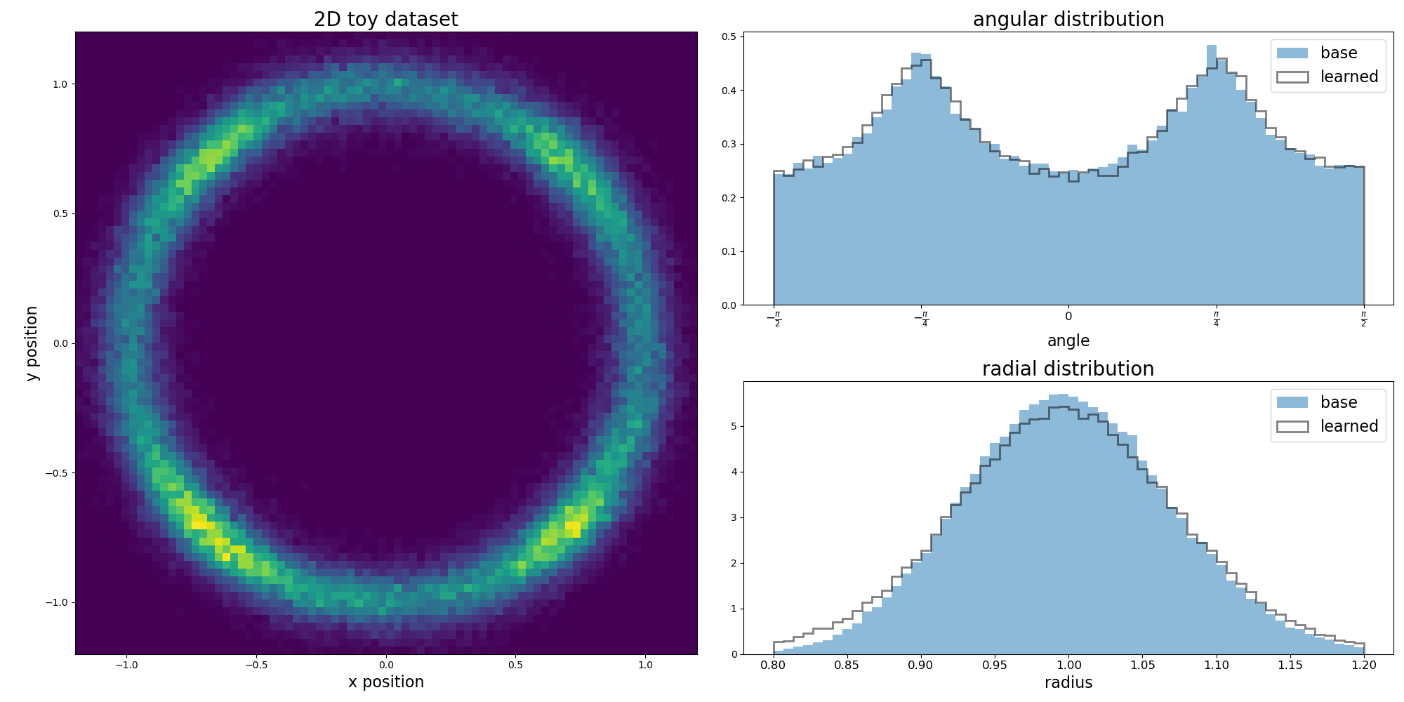 Toy dataset sampled from a learned diffusion model
Conclusions and improvements
-
Our toy diffusion model based on a vanilla feed-forward neural network learned the 2D dataset quite well. We did not need positional embedding or UNets.
-
Although diffusion models work quite well in the task of sampling, they tend to perform worse in recreating the overall data density (or finding the log-likelihood of the sample). To address this shortcoming, some authors suggested a possible way out based on the probability flow ODE.
-
The learning phase is simplified because the transition function \(p(x,t;x_0,0)\) is known explicitly. If the transition function is not known, in paper the authors propose a loss based on a sliced score.