Interested in AI? Heard of Smoluchowski? Have you stumbled lately on any breathtaking AI-generated images? Why am I asking you these questions? Find out here.
So there’s this guy…
So there’s this forgotten polish physicist, Marian Smoluchowski. In his short life he became one of the pioneers of statistical physics. One of his major achievements was to explain the erratic motion of pollen grain in water first reported by Brown:
 extracted from a clip
Why is it so strange? It seems that the grains move quite randomly due to interaction with the much smaller fluid particles… But hold on. Some context is urgently needed - as shocking as it sounds today, in the mid XIXth century, the existence of atoms themselves was a highly controversial idea! Some argue that Ludwig Boltzmann, the grandfather of statistical physics, took his own life because of brutal attacks against his microscopic, atomistic description of matter. If however there are no atoms, the fluid is a continuous, featureless medium and there is no reason for the erratic motion of pollen grains to happen. Still, as was shown by Smoluchowski, the motion is the net result of many interactions with small, invisible fluid molecules:
 simulation code
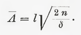
While he was not the only one to explain the motion (Einstein was also on it!), he embraced the atomistic perspective fully. In his seminal work, he derived a fundamental result for the average particle position changing as a square root of time:
This formula set out a number of further developments. The trembling motion is described fully by the Smoluchowski equation:
\[\frac{\partial}{\partial t} p_t(x) = D \frac{\partial^2}{\partial x^2} p_t(x)\]
where we restrict the motion to one dimension \(x\), \(D\) is a constant. Equation specifies \(p_t(x)\), the probability of finding a particle at \(x\) in time \(t\). The motion governed by this equation is known as the free diffusion since nothing is constraining the random motion.
Simulations
That was just the beginning of the story. Later, Langevin realized that single particles undergoing Brownian motion can be described in terms of a differential equation with an additional random (noise) function \(W(t)\):
\[\frac{d}{dt}x(t) = -ax(t) + \sqrt{2D} W(t)\]
This diffusive motion is constrained by a restoring force \(-ax\) keeping the particle from moving away to infinity (setting \(a=0\) takes us back to the free diffusion discussed previously). Langevin formulation is very easy to simulate, we approximate the derivative \(dx/dt \approx ( x(t+\delta t) - x(t) )/ \delta t\) and set time \(t = n \delta t\) while \(x(n\delta t) = x_n\) and \(W(n\delta t) \sqrt{\delta t} = W_n\):
\[x_{n+1} = (1- a \delta t ) x_n + \sqrt{2D} W_n \sqrt{\delta t}\]
The nontrivial part is a little bit of random function magic producing the square root \(\sqrt{\delta t}\). We simulate it for some initial position \(x_0\) and for \(N\) time-steps. It is instructive to compare single trajectories produced by the Langevin approach matched with the probabilistic description provided by the Smoluchowski equation:
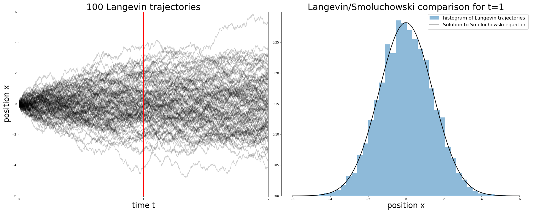 Comparison between (single-particle) Langevin equation and (probabilistic) Smoluchowski equation
In simulations we set the parameter \(a=0\), resulting in an unconstrained diffusive motion. Simulated trajectories are shown in the left plot up to time \(T = 2\). The right plot compares both approaches at fixed time \(t=1\) corresponding to a red vertical line on the left plot. The histogram is a result of binning the trajectories while the black line is an explcit solution to the Smoluchowski equation \(p_t(x) \sim \exp \left ( - x^2 / 4D t \right )\). Although the Langevin approach focuses on single trajectories while the Smoluchowski solution gives a global probabilistic picture, they are completely equivalent.
… But where is AI?
OK, it’s a nice story and all but… I came here because of the AI, what does it have to do with the cool stuff people do nowadays? Well, let’s look at the paper starting the newest generative craze “Denoising Diffusion Probabilistic Models” or the name Stable Diffusion. They happen to create truly breathtaking results:
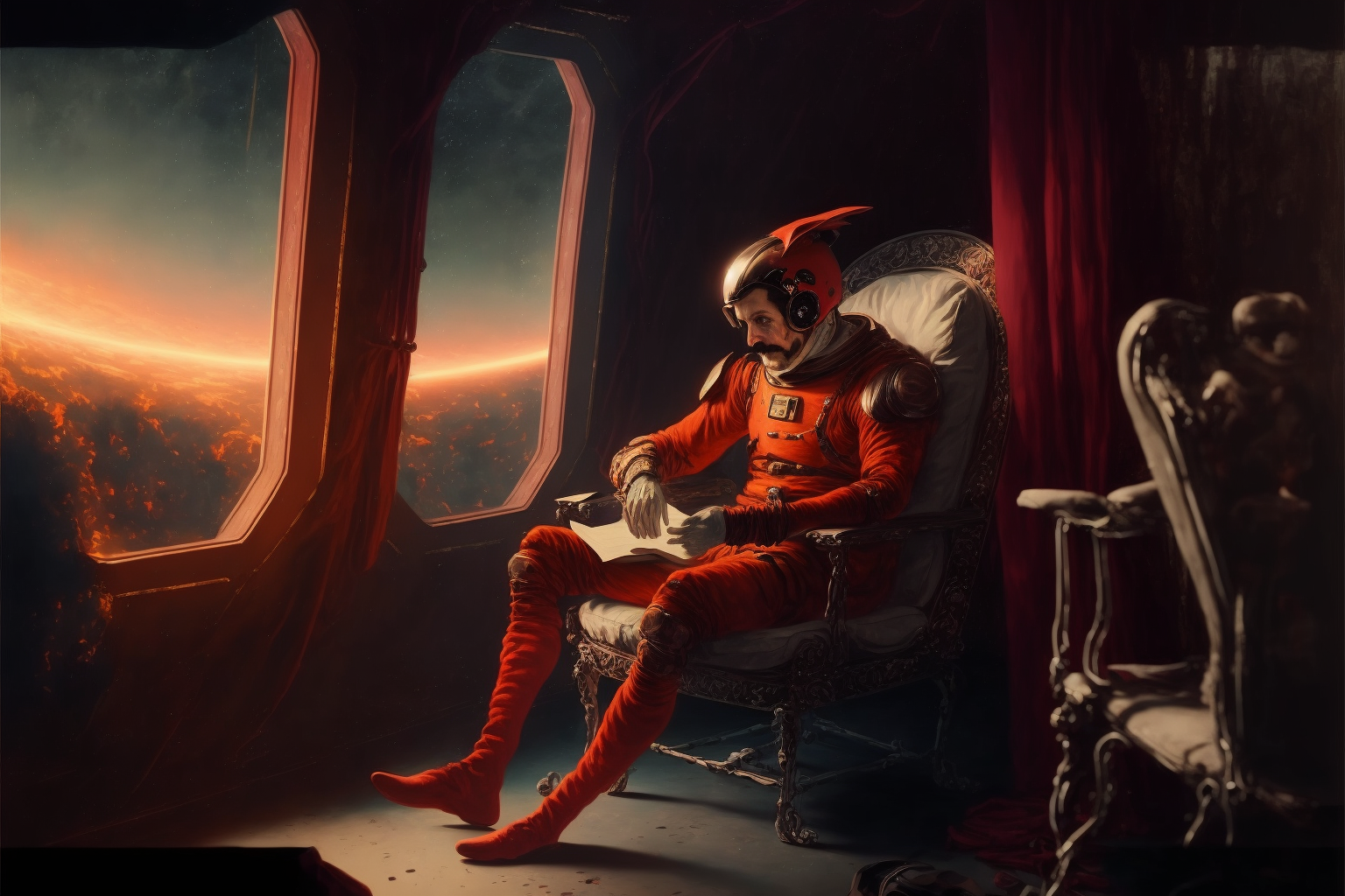 self-created using Midjourney
How is this possible? Simply put - it is precisely diffusion generalized to multiple dimensions which turns out to be quite powerful. There are two main parts of a generative diffusion model.
Forward process
We first define the so-called forward process – we take an initial image and gradually add noise to each pixel independently. In that way, we create a set of images with increasing levels of noise. The resulting equation is again:
\[\frac{d}{dt}x(t) = -ax(t) + \sqrt{2D} W(t)\]
where now \(x(t)\) denote the image pixels. Not focusing on minor details, when the final time \(T\) is large enough, the end result is a a pure Gaussian noise \(x(T) \sim N\left (0,\frac{D}{a} \right )\).
Reverse process
The key phase is to consider the reverse process coupled with the forward process. We start from complete noise and do a backward simulation to generate an image… But wait a second, how can this happen? After all, noise is featureless and thus lacks any initial information. That is true, that is why the Langevin equation for the reverse process contains an additional term:
\[\frac{d}{dt} x(t) = -ax(t) -2D \partial_{x(t)} \log p_t (x(t)) + \sqrt{2D} W(t), \qquad t \in (0,T)\]
Importantly, to solve this equation we need to go backward in time – starting from \(x(T)\) and evolve it back to \(x(0)\)! This is not how you typically solve an initial value problem for differential equations but nothing forbids us from doing so.
But what is the extra term? The driving function \(\partial_{x} \log p_t (x)\) (aka the score function) is the (derivative of the log-) marginal probability for the forward process… Or what exactly? A known fundamental solution \(p(x,t; x_0,0)\) (of the Smoluchowski equation!) integrated over the initial distribution \(p_0\):
\[p_t(x) = \int dx_0 p_0(x_0) p(x,t; x_0,0).\]
Neural network
We defined both the forward and reverse processes as intimately related but… It looks like we reached an impasse - a backward process which could help us to sample from \(p_0\) has an extra term which depends on the density we aim to sample from!
This is where the ML magic enters - we need an expressive score function in order to drive an initial pure-noise picture into something resembling an image. A neural network \(s_\theta(x(t),t)\) will do this job.
Learning the score function \(s_\theta\)
If there’s a neural network, it needs a learning objective. In our case, the learning minimizes the following loss function
\[L(\theta) = E_{t\sim U(0,T)} E_{x(0)} E_{x(t)| x(0)} \left ( \lambda(t) \left \| s_\theta(x(t),t) - \partial_{x(t)} \log p(x(t), t; x(0),0) \right \|^2 \right )\]
where the expectation values are taken over
- time \(t\) (drawn from a uniform distribution)
- initial images \(x(0)\) (the images from the dataset to be learned)
- noisy images \(x(t)\) at time \(t\) resulting from \(x(0)\) (generated by the forward process)
The transition kernel \(p(x, t; x_0,0)\) is a fundamental solution to the Smoluchowski equation (can be calculated explicitly) while \(\lambda(t)\) is the time-weighting function. The learning objective is to find a neural network matching the transition kernel score for each time \(t\) and noisy image \(x(t)\):
\(s_\theta(x(t),t) \approx \partial_{x(t)} \log p(x = x(t), t; x=x(0),t=0)\)
Image generation
Output of the training phase is the optimal score function \(s_{\theta_*}\). It is used in the generative reverse process. Because it evolves backward in time, we use the retarded approximation to time derivative \(dx/dt \approx ( x(t) - x(t-\delta t))/ \delta t\) and the discretized Langevin equation reads
\[x_{n-1} = (1 + a \delta t) x_n - s_{\theta_*}(x_n,n\delta t) \delta t + \sqrt{2D} W_n \sqrt{\delta t}, \quad n = N,N-1,...,1 .\]
where the initial value \(x_N = x(T)\) is drawn from the normal distribution. If the learning process was succesful, the end result is a sample \(x_0\) drawn from the learned image distribution.
Conclusions
-
Diffusion explained the motion of pollen grain and strengthened the atomistic viewpoint. Diffusive process have two equivalent descriptions in terms of Langevin equation (microscopic) and a Smoluchowski equation (macroscopic).
-
Diffusion models considerd in machine learning consist of a learnable score function (typically a neural network) and a noise-adding process. The learning process optimizes the network to match the noise-adding process executed on the learned dataset.
-
Pollen grain to computer-aided image generation, what a journey!