
Diffusive models provide good results when it comes to sampling the learned data. Unfortunately, most of the out-of-the-box solutions cannot access the underlying data likelihood. In this post we discuss ways to overcome it. Code is provided.
Recap
In part 2 of the series on diffusion models, I described the fundamental mechanisms with the help of 2D synthetic data. The model consists of learning a score function and then solving the Langevin equation to sample new data. I provide a simple nano-diffusion code with a feed-forward neural network serving as the approximate score function.
Finding the likelihood
Although diffusion models have clear advantages, I now turn to discussing its limitations and ways of overcoming them. Besides often quoted relative slowness of the sampling process, the lack of direct access to data likelihood is a major disadvantage. In this part, I discuss ways of addressing this limitation.
In part 2, probability densities were found by simply plotting histograms of many samples which is clearly unfeasible for higher dimensions. Another, less straightforward approach is to use a description complementary to the Langevin and Smoluchowski equations known as the probability flow equations. I will discuss it in this post.
Probability flow equation
The probability flow equation is a representation for a forward process fully equivalent to the Langevin and Smoluchowski. For the forward process of the form
\[\frac{d}{dt} x(t) = f(x(t),t) + g(t) W(t),\]
there exists an equivalent description in terms of the probability flow equation:
\[\frac{d}{dt} x(t) = f(x(t),t) - \frac{1}{2} g(t)^2 \partial_{x(t)} \log p_t(x(t)).\]
The intriguing fact is the random term \(\sim W(t)\) is traded for an additional determininistc part \(\sim \partial_x \log p_t(x)\) containing the score function. This is the same score function present in the backward process introduced in part 2 of the series.
But where’s the probability which flows? Well, you can recast above equation into a probabilistic form:
\[\frac{d}{dt} \log p_t(x(t)) = - \text{Tr} \partial_{x(t)} \tilde{f}(x(t),t),\]
where \(\tilde{f}(x(t),t) = f(x(t),t) - \frac{1}{2} g(t)^2 \partial_{x(t)} \log p_t(x(t))\) is the r.h.s. of the previous equation. The \(\text{Tr}\) is a trace operation because \(\partial_{x(t)} \tilde{f}(x(t),t)\) is a matrix. Crucially, this equation has the \(\log p_t\) term on both sides.
For practical purposes, we put both equations into a single form:
\[\frac{d}{dt} \left ( \begin{array}{c} x(t) \\ \log p_t(x(t)) \end{array} \right) = \left ( \begin{array}{c} \tilde{f}(x(t),t) \\ - \text{Tr} \partial_{x(t)} \tilde{f}(x(t),t) \end{array} \right) .\]
In this form, the equations are implicit as the \(\log p_t\) function is present on both sides.
Training procedure
The training procedure is the same as in the part 2 where a synthetic 2D dataset was recreated. That happens since the probability flow equations contain the same score function as the one found in the Langevin backward process. Therefore, to train a diffusion model it suffices to find an approximate score function \(s_\theta\) in the usual way and then plug into the probability flow equations.
The minor differences in the training procedure is in a different choice of the \(\lambda(t)\) weighting function which is now given by \(\lambda(t) = \beta(t)\). This choice is dictated by a mismatch between the training objectives - to obtain the best samples or to obtain the best likelihood. We also take a nonzero initial time \(t = T_\epsilon > 0\) to not deal with the instabilities near \(t = 0\).
Probability flow on a toy dataset
I provide code to this part. To show the probability flow approach in action, I take a simple 1D dataset (a mixture of 3 Gaussians). The training procedure is discussed previously so we do not focus on it and instead move on to finding the likelihood. The probability flow equation is solved in two ways which we discuss in detail below.
The likelihood via probability flow
Numerical integration of the probability flow equation is used to calculate the data likelihood \(\log p_0(x(0))\):
\[\log p_0(x(0)) = \log p_T(x(T)) + \int_0^T dt \text{Tr} \left ( \partial_{x(t)} \tilde{f}(x(t),t) \right ).\]
The implementation is given below:
def likelihood_ode(score_net, x_low = -4., x_high = 4., x_npts = 10000):
    '''
    likelihood via probability flow equation (ODE)
    '''
    def gen_score_net_div(score_net):
        def score_net_div(x,t):
            x.requires_grad_(True)
            model_output = score_net(x, t)
            model_div = torch.autograd.grad(torch.sum(model_output), x, create_graph=True)[0]
            x.requires_grad_(False)
            return model_div

        return score_net_div

    def gen_ode_likelihood(init_x: np.ndarray, rtol=1e-5, atol=1e-5, method='RK45'):

        def ode_func(x, t):
            return -0.5 * beta(t) * ( x + score_net(x, t))

        def ode_func_div(x, t):
            return -0.5 * beta(t) * ( 1 + score_net_div(x, t))

        def prior_logp(z):
            logZ = -0.5 * np.log(2 * np.pi)
            return (logZ - 0.5 * z**2).sum(axis=1, keepdims=True)

        def x_logp_ode_solver_func(t: float, x_logp: np.ndarray):

            x = torch.from_numpy(x_logp[:x_npts*x_dim].reshape(x_npts,x_dim))
            x = x.to(device).float()
            t = (torch.ones(x_npts, 1).to(device) * t).requires_grad_(False)

            drift = ode_func(x, t).reshape(-1).detach().cpu().numpy()
            logp_grad = ode_func_div(x, t).reshape(-1).detach().cpu().numpy()

            return np.concatenate([drift,logp_grad],axis=0)

        x_npts,x_dim = init_x.shape
        init_x_logp = np.concatenate([init_x.reshape(-1),np.zeros(x_npts)],axis=0)
        solution = scipy.integrate.solve_ivp(x_logp_ode_solver_func,
                                             (Teps,T),
                                             init_x_logp,
                                             rtol=rtol,
                                             atol=atol,
                                             method=method,
                                             t_eval = np.linspace(Teps,T,100))

        t = solution.t
        sol = solution.y[:, -1]
        x = sol[:x_npts*x_dim].reshape(x_npts,x_dim)
        logp = sol[x_npts*x_dim:].reshape(x_npts,1)

        logpT = prior_logp(x) # log(p(x(T)))
        logp = logpT + logp

        return logp

    score_net_div = gen_score_net_div(score_net)

    init_x = np.linspace(x_low,x_high,x_npts)
    init_x = np.expand_dims(init_x,-1)
    logp = gen_ode_likelihood(init_x = init_x)

    return init_x, logp
where we use the integrator scipy.integrate.solve_ivp to find the integral. The initial term \(\log p(x(T))\) is calculated explicitly from the Gaussian distribution. The likelihood is a result of evolving \(10000\) equidistant points between \((-4,4)\) from \(t = T_\epsilon\) up to \(t = T\).
Sampling via probability flow
The probability flow equations can also be used to obtain data samples. We solve it with the help of time discretization and obtain a number of samples from the approximated data distribution \(p_0\).
Likelihood and sampling comparison
The comparison of sampling and explicit likelihood calculation are shown below:
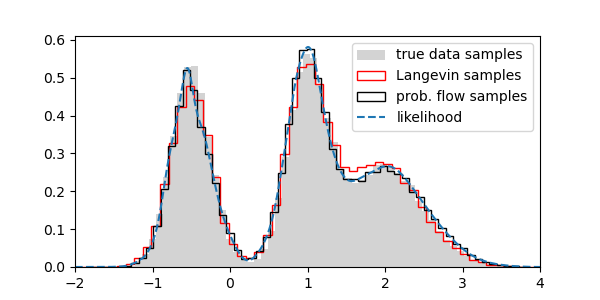 Likelihood
Both sampling aproaches follow closely the ground truth data. The likelihood function also behaves similarly to the data.
It is instructive to show time-resolved solutions to the Langevin and probability flow equations to spot the differences:
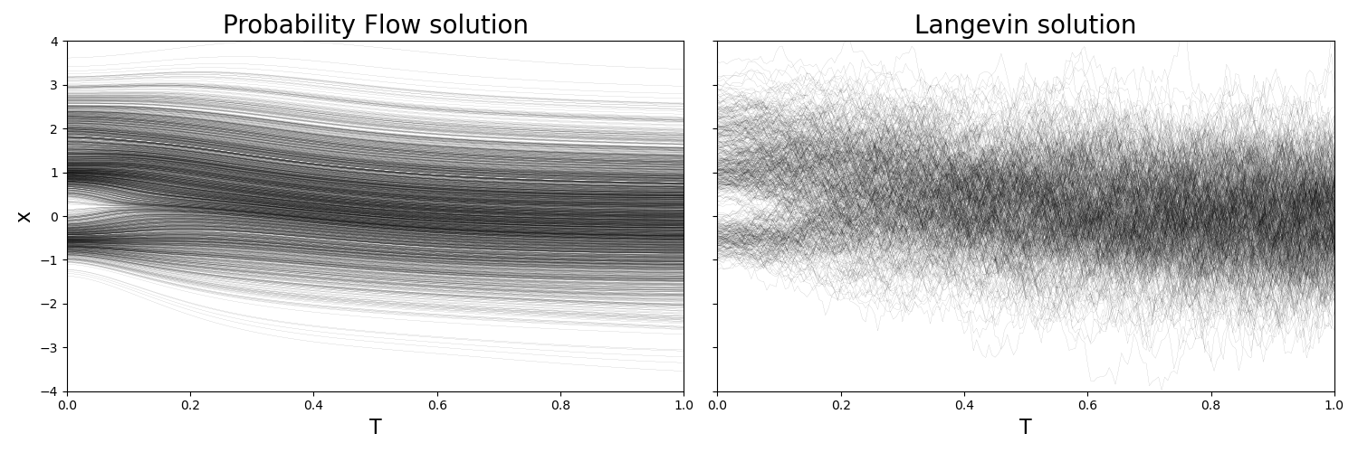 Solutions
where the stochastic term present in the former is really driving the erratic behavior. Still, the equal time probability densities agree quite well.
Possible extensions
A natural extension of this approach is signalled in the approximation step - the r.h.s. of the probability flow equation depends on the score function and therefore can be expanded beyond the score function. In that way, the higher order score function terms show up which can in turn be learned by score matching techniques. This was done up to the third order in.
Conclusions
- Probability flow equations enable explicit calculations of the learned data likelihood. The results on 1D dataset clearly show that the method works.
- Using probability flow is possible with the approximate score function neural network so that no retraining of the diffusion model is needed.
- Although additional training is not mandatory, small changes in the weight function tend to improve the likelihood estimation. There exists also more involved methods to improve by looking at higher order score functions or improving the training stability via importance sampling.