
What is arbitrage? Has it gone extinct in the modern age? How to spot it in the wild? Is there any physics involved?
Arbitrage? Quepasa?
Although the term “arbitrage” may sound unfamiliar, it represents a Holy Grail in the world of speculative investing - the quest for risk-free profit through the exploitation of pricing disparities across markets. To illustrate the concept, consider a foreign exchange market that includes five currencies: PLN, USD, EUR, CHF, and JPY. Suppose you possess 100 PLN and are actively seeking out potential arbitrage opportunities. Rather than the typical investment approach of buying, holding, and selling, you instead aim to complete an instanteneous cycle of currency exchanges that both starts and ends with the currency you hold. Below, we provide an example of a four-step arbitrage cycle involving PLN as one of the nodes:
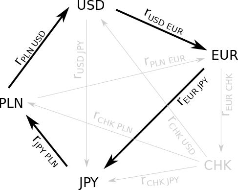
To begin the arbitrage cycle, you would first exchange your PLNs for US dollars, followed by purchasing EUR, then JPY, and finally ending with the acquisition of PLNs once again. The ultimate question is, how much profit can be made? In an ideal world, the answer is straightforward - there should be no profit gained, and in fact, there may be a loss due to the incurred exchange fees. This expectation is rational and probable, but it is based on the assumption of a market that operates efficiently or is free of arbitrage opportunities.
My objective is twofold. First, to illustrate the occurrence of arbitrage in real-world scenarios. While it is one thing to learn about it from a textbook, observing these mechanisms in action through actual data is a different experience altogether. Second, I show that exotic investments sometimes offer more profitable outcomes. To accomplish this, I examine arbitrage opportunities in the simplest case of the foreign exchange market.
Arbitrage function
Before delving into the results, let us first introduce some notation to define the arbitrage function \(A\). We will use the notation \(r_{i,j}\) to represent the exchange rate between currencies i and j. For instance, if \(r_{PLN,USD} = 4.50\), it means that 1 US dollar (USD) is equivalent to 4.50 Polish zlotys (PLN) on a given trading day. The arbitrage term can then be expressed as a straightforward product of \(N\) rates (where \(N\) is the length of the arbitrage cycle):
\begin{equation}
r_{PLN,j} ~ r_{j,k} ~ r_{k,l} \cdots r_{x,PLN},
\end{equation}
where one of the nodes in the arbitrage cycle is the currency that we possess (in this case, PLN). For the time being, we will disregard the time dimension and assume that all transactions take place within a single day. The success (or failure) of the arbitrage cycle is determined by whether it yields a value greater (or smaller) than one. The arbitrage function \(A\) can be expressed as follows:
\begin{equation}
A_{PLN} = r_{PLN,j} r_{j,k} r_{k,l} … r_{y,x} r_{x,PLN} - 1.
\end{equation}
This function calculates the realized gain (positive) or loss (negative) resulting from the arbitrage cycle, with PLN being the base currency. Notably, our approach does not consider any transaction fees that may be incurred during the process.
The data
To conduct the analysis, I obtained four years’ worth of daily forex data using an unofficial Yahoo Finance Python package called yfinance. I collected data for all available pairs of the top 25 most traded currencies. Next, I computed the arbitrage functions for 3- and 4-step arbitrage cycles that included the PLN base currency. An example of a typical well-behaved arbitrage function between major currencies is depicted in the graph below:
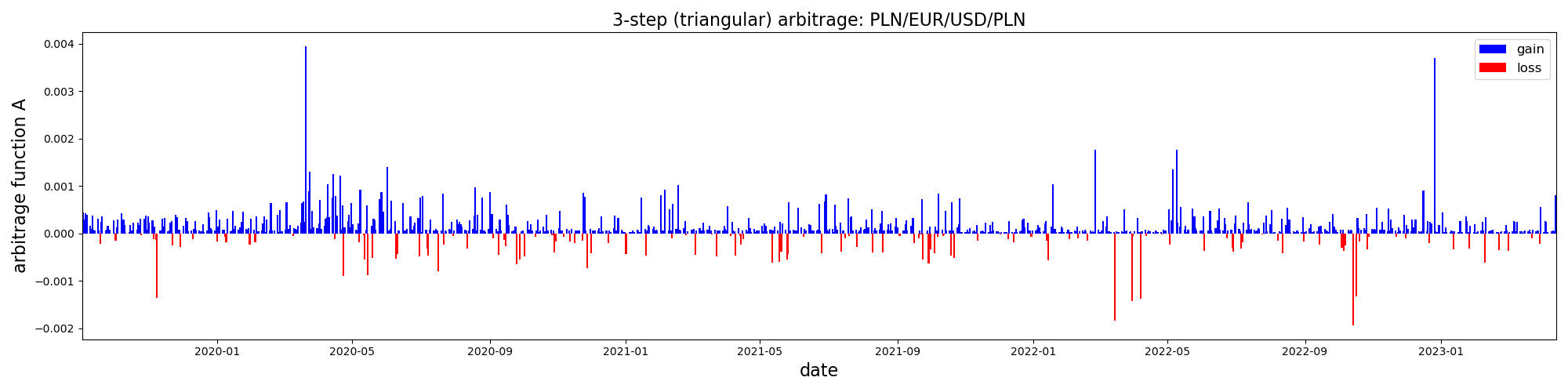
In this case, we observe an almost negligible effect, with a value of approximately \(0.01\%\), relatively few outliers and limited arbitrage opportunities. However, it is important to note that not all cycles exhibit such behavior. As an extreme example, consider the following scenario in which the arbitrage opportunity is much more pronounced:
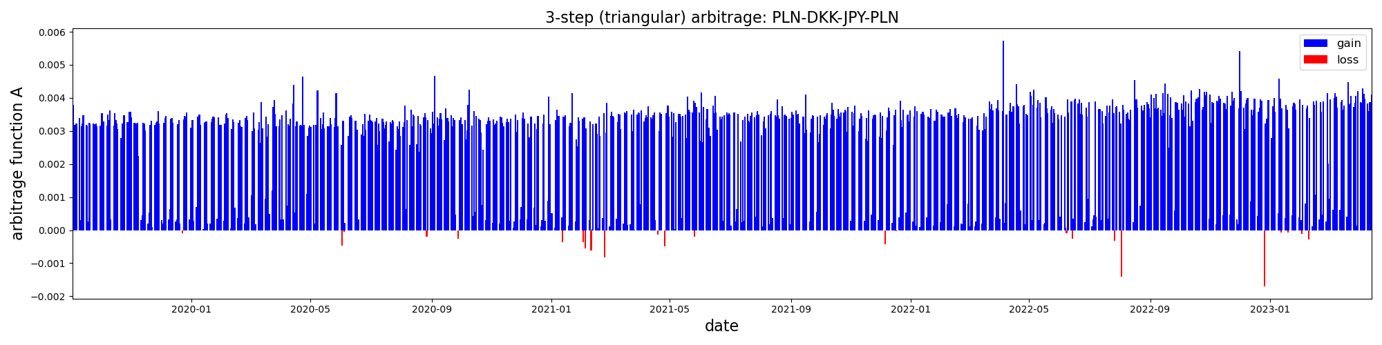
In this case, the average effect is much more significant, reaching approximately \(0.3\%\). Does this indicate that we have discovered something noteworthy? It’s difficult to say for certain, but it certainly appears intriguing. The distribution of arbitrage values is quite bimodal, with one peak centered around zero and the other around the aforementioned \(0.3\%\) value. I examined the remaining cycles and identified several other promising arbitrage scenarios. In the figure below, I have presented the mean arbitrage outcomes with associated statistical errors, with cycles ordered based on their mean potential gains:
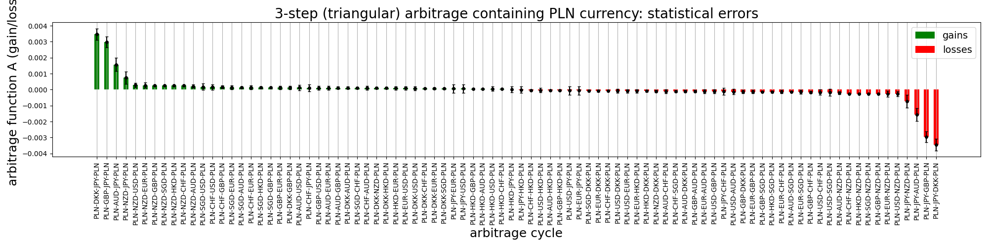
The four top performing arbitrage cycles include the Japanese yen JPY. It is possible that these results are due to the yen being a relatively highly-denominated currency, which means that you can buy a lot of yen for relatively few euros. However, the values of exchange rates are relative, so currency denominations should not matter. However, in the search for arbitrage opportunities, we consider multiplications of random numbers and their deviations from unity, which can compound and produce a arbitrage function with high variance. While this is generally true, we see a distinctly bimodal distribution of \(A\)’s for JPY-related arbitrage cycles, which remains unexplained. Another possibility is that the rates data could have been rounded to such an extent that quantization effects are observed. However, this is unlikely as we observe the same type of bimodality in JPY-containing cycles based on the euro.
Other examples
In the case of the base currency EUR, we have found that not all arbitrage cycles exhibit stationary behavior:
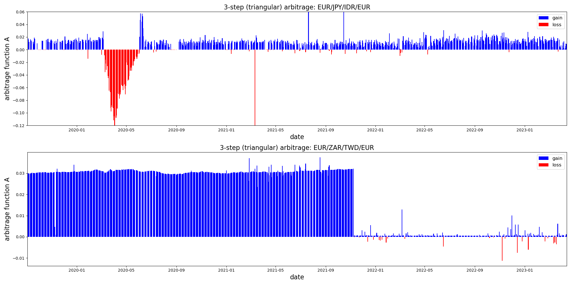
The previous case lacked exchange rates with more exotic currencies, whereas here we can clearly see that the Western markets provide fewer arbitrage opportunities with lower gains. This can be easily understood as the Western economies are better connected and adhere more closely to the efficient market assumption. On the other hand, connecting to Eastern markets tend to produce higher gains and more volatility.
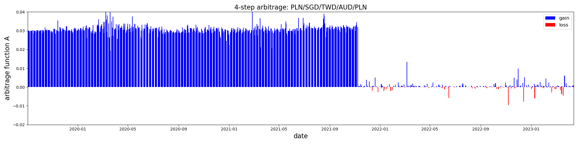
Four-step arbitrage
Expanding beyond triangular arbitrage is a straightforward process. However, it may not necessarily lead to genuinely new paths, but rather give access to existing ones due to the limited availability of currency pairs. Let me explain this using an example. When considering 3-step arbitrage containing the PLN currency, we were unable to reach the TWD currency due to a lack of currency pairs. As a result, any potentially profitable triangular arbitrage cycles could not pass through both TWD and PLN. We chose the TWD currency because of a distinctive step-like shape of the arbitrage curve that ended around Nov 2021, as shown in the previous plot. Extending the arbitrage path by one step allowed us to tap into this opportunity. In the figure below, I present the best performing 4-step arbitrage with PLN as the base currency. In accordance with our observation, it now passes through the TWD currency and exhibits a similar step-like behavior.
Our approach uses single-day data, which means that the entire arbitrage cycle should be executed within that day. Ideally, we aim for instantaneous execution, as that is the implicit assumption of arbitrage. However, executing arbitrage “in time” is also possible but it requires the use of futures contracts, so that the full loop is “executed” simultaneously.
Interestingly, arbitrage also has a strong connection with physics. The assets (like currencies) are interpreted as points of a discretized space-time while the electromagnetic potential located on the links between the space-time points are the exchange rates. In this language, denomination of the currencies is a local symmetry. The no-arbitrage assumption can be interpreted geometrically as a pure-gauge configuration of the electromagnetic field. The connection goes quite far as the equal-time arbitrage cycles are the analog of the magnetic fields, while arbitrage involving time (with futures contracts) can be viewed as the electric field.
Conclusions
- We identified several promising 3-step JPY-related arbitrage opportunities (PLN/DKK/JPY/PLN) with a steady \(0.3 \%\) ROI.
- Our analysis confirms that arbitrage exists even in the liquid forex market.
- The profitability of arbitrage depends on the development and connectedness of markets.
- Promising arbitrage opportunities can be short-lived and end abruptly, so vigilance is key.