
In the real world, time series data tend to be a) nonstationary and b) periodic or quite periodic. We discuss how Fourier transform helps in both controling and understanding the typical methods of seasonal decomposition of time series. Code provided.
Majority of materials on time series seasonal-trend decomposition focus on listing different approaches but lack tools to understand them. In this short note I use Fourier methods to pinpoint the differences between classic decomposition methods and discuss the impact of control parameters on the Fourier spectra of each decomposition method.
Our working example
We consider a publicly available time series data
of hourly traffic at a junction.
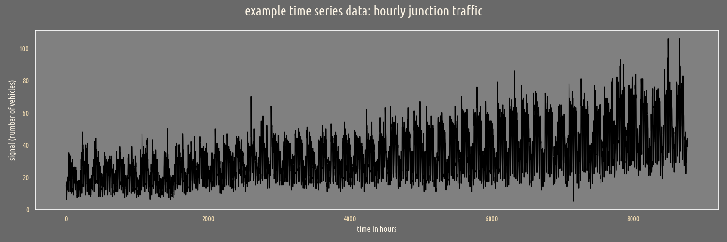
Data is gathered every hour, we can clearly discern daily and weekly changes. Such periodic changes are extracted with the help of popular seasonal decomposition tools implemented in the statsmodels python package. A table summarizing decomposition approaches:
statsmodels name |
trend extraction method |
# seasonal signals |
seasonal periodicity |
trend scale parameter |
seasonal period param |
seasonal period relaxation param |
seasonal_decompose |
moving average |
1 |
fixed |
period |
period |
N/A |
STL |
LOESS |
1 |
relaxed |
trend |
period |
seasonal |
MSTL |
LOESS |
>1 |
relaxed |
trend via stl_kwargs |
periods |
windows |
Main differences between these methods are:
- exact or relaxed periodicity of the seasonal part
- decomposition into multiple seasonal signals (MSTL)
- specification of the trend signal time-scale
We use Fourier analysis to clearly present these differences.
Fixed-period seasonality: seasonal_decompose
Additive model is decomposed into three parts: trend T, seasonal change S and noise N:
\[X(t) = T(t) + S(t) + N(t)\]
The trend is the slowly varying component, seasonal signal is the periodic part while the noise is the residual part.
At first we take into account the weekly seasonality change and set period = 24*7:
from statsmodels.tsa.seasonal import seasonal_decompose

period = 24*7
sd = seasonal_decompose(x, period = period, extrapolate_trend = 'freq')
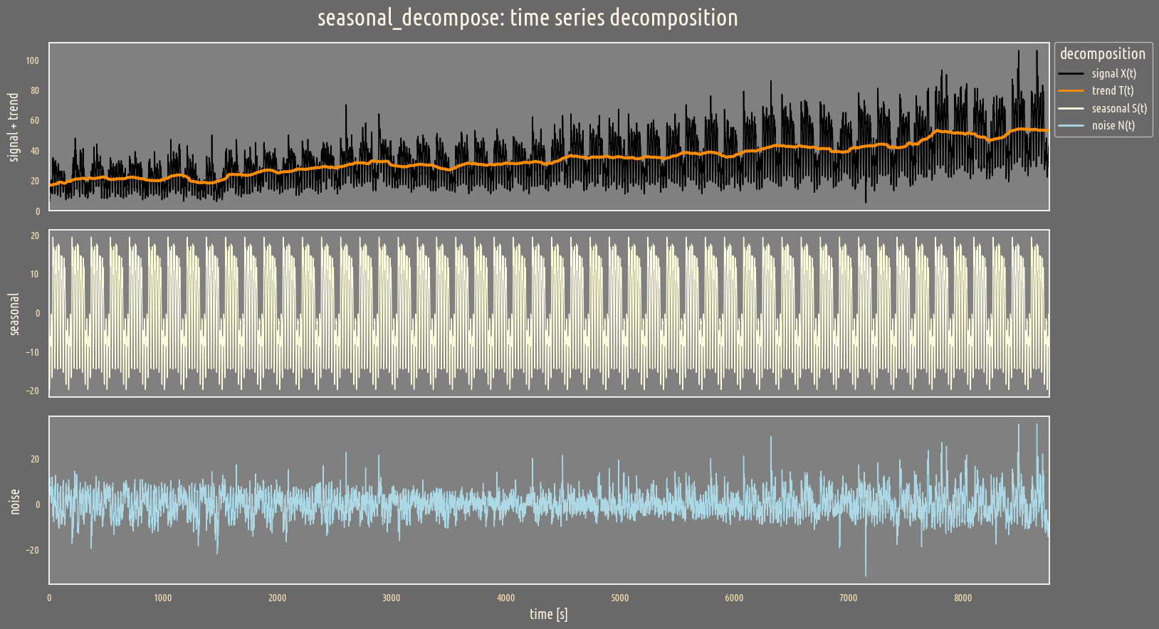
Clearly the trend and seasonality is decoupled. But how does it work in detail?
The crucial parameter of the seasonal_decompose function is the integer period specifying two features of the decomposition:
- the characteristic period of the seasonal signal and,
- the time scale boundary above which the trend is defined.
The power spectrum for each part of the decomposed signal is shown below.

First, the trend is dominant (has the largest power) in the band below the seasonal fundamental frequency 1/period denoted by a thick, dashed vertical line. The seasonal signal is in turn dominant only near multiplicities of the seasonal fundamental frequency.
Almost-fixed-period seasonality: STL
\[X(t) = T(t) + \tilde{S}(t) + N(t)\]
$\tilde{S}$ represents the seasonal part whose period is centered around a single value.
Code for the application of the STL decomposition:
from statsmodels.tsa.seasonal import STL

period = 24*7
trend = period*2 + 1
seasonal = 7
stl = STL(endog = x,period = period,trend = trend,seasonal = seasonal)
stl = stl.fit()
The result is shown below:
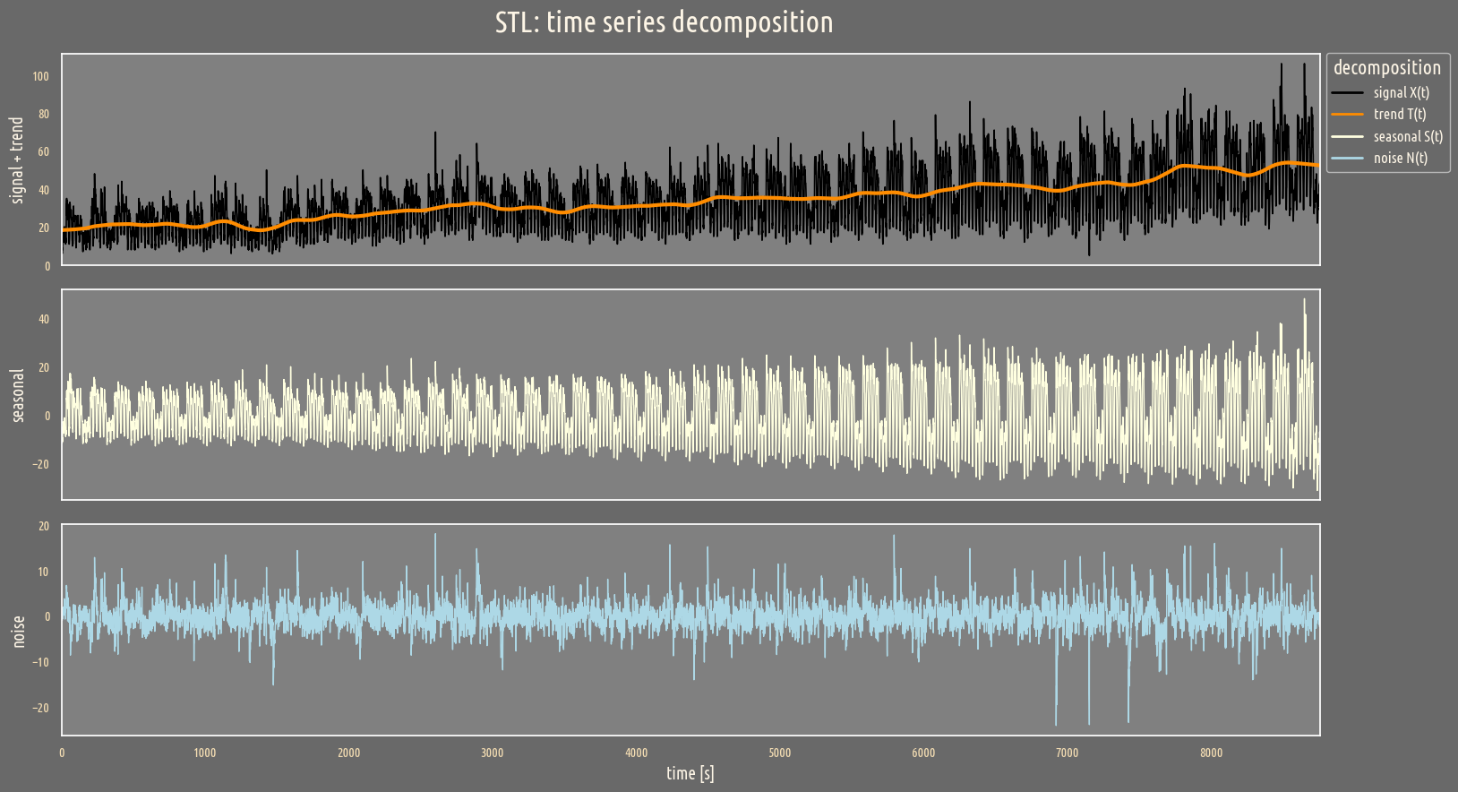
In comparison to the previous case, the seasonal part has more aperiodic structure. The amount of this aperiodicity is controlled by the seasonal parameter. Secondly, the trend parameter is a cutoff above which the signal is interpreted as a trend. In the previous decomposition, the trend cutoff was equal to the fundamental period period = trend.

The relaxation of the seasonality period is evident by the power increase in the vicinity of each multiplicity of the fundamental frequency 1/period. This relaxation of the seasonality period is controlled by the seasonal parameter. Moreover, a trend cutoff frequency 1/cutoff controls which part
of the signal spectrum is considered as the trend part.
Analysis of both methods is easier on the component-wise comparison of Fourier spectra for both methods:
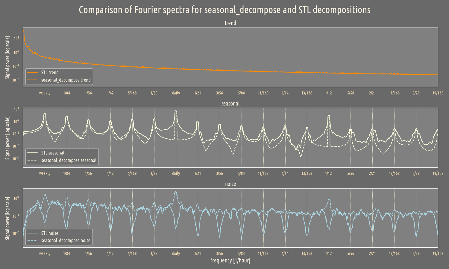
The trend line remains the same while the spectra for seasonal and noise parts point toward a change in the interpreration of the detrended signal - in STL more noise is taken as the seasonal signal.
Multiple seasonalities: MSTL
So far we have focused on a weekly seasonality but our data contains one more obvious period - the 24-hour period. How to deal with that? MSTL comes to the rescue.
In general, the signal now contains n_s seasonal parts:
\[X(t) = T(t) + \sum_{i=1}^{n_s} \tilde{S}_i(t) + N(t)\]
In this case, we have a list of periods for each seasonal component and a set of relaxation parameters windows (confusingly these correspond to the seasonal parameter in the STL method).
from statsmodels.tsa.seasonal import MSTL

periods = [24,24*7]
trend = max(periods)*2+1
windows = [7, 7]
mstl = MSTL(endog = x,periods = periods, windows= windows, stl_kwargs = dict(trend = trend))
mstl = mstl.fit()
Besides the weekly seasonality considered previously, we set an additional daily period = 24.
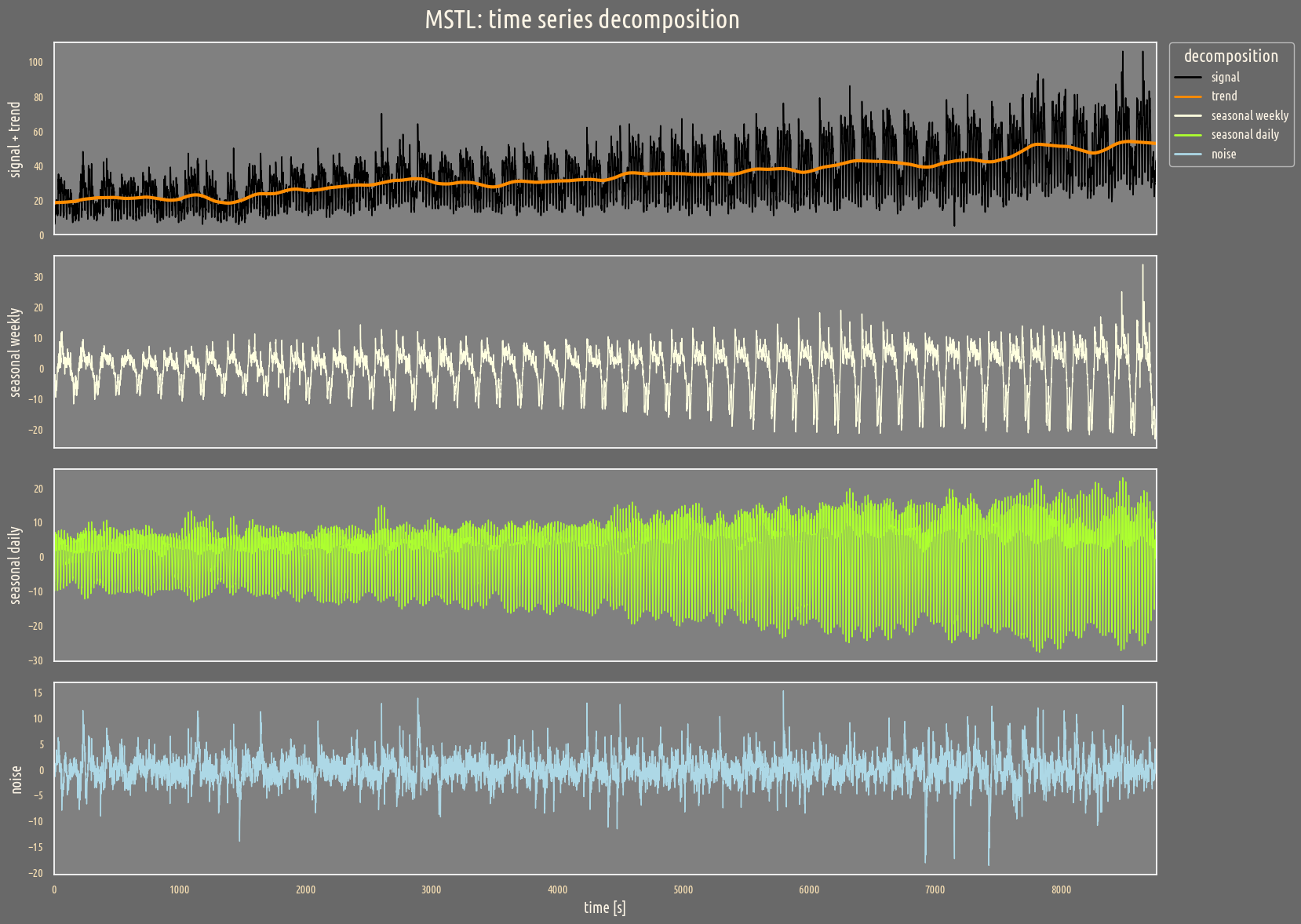
Additional seasonal signal is captured. What about the Fourier spectrum?
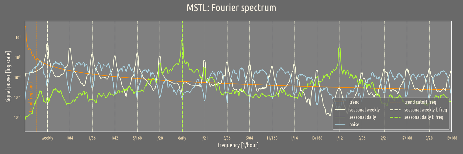
It behaves similarly as to the STL spectrum but now, the additional daily period has the largest power near the period = 1/24.
Conclusions
- Fourier analysis reveals a clear picture of seasonality decomposition of time series data.
- Main parameters for each considered method have clear implications on the power spectrum.